Section 5 Quantifying Uncertainty

In almost any archaeological network study, the networks we create are incomplete (i.e., we know that we are missing nodes or edges for various reasons: site destruction, lack of survey coverage, looting, etc.). How might the fact that our networks are samples of a larger and typically unobtainable “total network” influence our interpretations of network structure and node position? In this section, we take inspiration from recent research in other areas of network research (Borgatti et al. 2006; Costenbader and Valente 2003; Smith and Moody 2013; Smith et al. 2017; Smith et al. 2022) and develop a means for assessing the impact of missing and poor quality information in our networks. This accompanies Chapter 5 of Brughmans and Peeples (2023) and we recommend that you read Chapter 5 as you work through the examples below.
For most of the other analyses presented in the book it is possible to use a number of different network software packages to conduct similar analyses. The analyses presented in Chapter 5, however, require the creation of custom scripts and procedures that are only possible in a programming language environment like R. We attempt here to not only provide information on how to replicate the examples in the book but also provide guidance on how you might modify the functions and code provided here for your own purposes.
5.1 R Scripts and Custom Functions
In this chapter, we have created a number of relatively complex custom functions to conduct the assessments of network uncertainty outlined in Chapter 5. We provide step by step overviews of how these functions work below but it is useful to bundle the functions into .R script files and call them directly from the file when working with your own data.
The scripts described in detail below include:
- sim_missing_nodes.R - Assessments of the stability of centrality metrics for networks with nodes missing at random or due to a biased sampling process.
- sim_missing_edges.R -Assessments of the stability of centrality metrics for networks with edges missing at random or due to a biased sampling process.
- sim_missing_inc.R - Assessments of the stability of centrality metrics for networks with nodes missing at random or based on biased sampling from incidence matrix data.
- sim_target_node.R - Assessments of the stability in rank order position of a target node in networks with nodes missing at random or due to a biased sampling process.
- sim_samp_error.R - Assessments of the stability centrality metrics due to sampling error in frequency data underlying similarity networks.
- edge_prob.R - Functions for conducting edge probability modeling and plotting candidate networks and centrality distributions.
Each of these are described in greater detail below along with an example. To run these scripts in R, you need to put them in your working directory and then use the source() function. The source function will run all code within the .R file and initialize any functions they contain. For example:
source("scripts/sim_missing_nodes.R")Note that you must include the correct absolute or relative file path for the script to run properly.
5.2 A General Approach to Uncertainty
As outlined in the book, our basic approach to quantifying and dealing with uncertainty is to use the sample we have as a means for understanding the robustness or vulnerability of the population from which that sample was drawn to the kinds of variability or perturbations we might expect. The procedures we outline primarily take the following basic form:
- Define a network based on the available sample, calculate the metrics and characterize the properties of interest in that network.
- Derive a large number of modified samples from the network created in step 1 (or the underlying data) that simulate the potential data problem or sampling issue we are trying to address. For example, if we are interested in the impact of nodes missing at random, we could randomly delete some proportion of the nodes in each sample derived from the network created in step 1.
- Calculate the metrics and characterize the properties of the features of interest in every one of the random samples created in step 2 and assess central tendency (mean, median) and distributional properties (range, standard deviation, distribution shape, etc.) or other features of the output as appropriate.
- Compare the distributions of metrics and properties (at the graph, node, or edge level) from the random samples to the “original” network created in step 1 to assess the potential impacts of the perturbation or data treatment. This comparison between the properties of the network created in step 1 and the distribution of properties created in step 3 will provide information directly relevant to assessing the impact of the kind of perturbation created in step 2 on the original network sample and, by extension, the complete network from which it was drawn.
The underlying assumption of the approach outlined here is that the robustness or vulnerability to a particular perturbation of the observed network data, drawn from a total network that is unattainable, provides information about the robustness or vulnerability of that unattainable total network to the same kinds of perturbations. For example, if we are interested in exploring the degree distribution of a network and our sampling experiments show massive fluctuations in degree in sub-samples with only small numbers of nodes removed at random, this would suggest that the particular properties of this network are not robust to nodes missing at random for degree calculations. From this, we should not place much confidence in any results obtained from the original sample as indicative of the total network from which it was drawn. On the other hand, say we instead find that in the resampling experiments the degree distributions in our sub-samples are substantially similar to that of the original network sample even when moderate or large numbers of nodes are removed. In that case, we might conclude that our network structure is such that assessments of degree distribution are robust to node missigness within the range of what we might expect for our original sample. It is important to note, however, that this finding should not be transferred to any other metrics as any given network is likely to be robust to certain kinds of perturbations for certain network metrics, but not to others.
5.3 Nodes Missing at Random
This sub-section accompanies the discussion of nodes or edges missing at random in Brughmans and Peeples (2023) Chapter 5.3.1. Here we take one interval of the Chaco World ceramic similarity network (ca. A.D. 1050-1100) and simulate the impact of nodes missing at random on network centrality statistics. Download the ceramic similarity adjacency matrix to follow along.
The first thing we need to do is initialize our required libraries, import the network adjacency matrix, and convert it into a igraph network object. For several of the examples in this section we are using a simple undirected network though the code would also work for weighted or directed networks as well.
library(igraph)
library(reshape2)
library(ggraph)
library(ggpubr)
library(statnet)
# Import adjacency matrix and covert to network
chaco <- read.csv(file = "data/AD1050net.csv", row.names = 1)
chaco_net <- igraph::graph_from_adjacency_matrix(as.matrix(chaco),
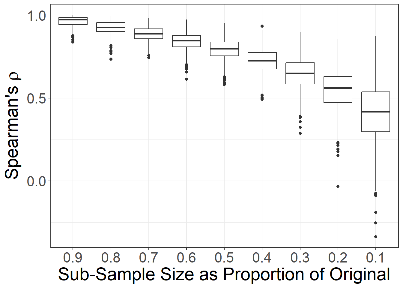
mode = "undirected")First, following Chapter 5.3.1, we will assess the robustness of these data to nodes missing at random for betweenness and eigenvector centrality. In order to do this we need to define a function that removes a specified proportion of nodes at random, assesses the specified metric of interest, and compares each sub-sample to the original sample in terms of the rank order correlation (Spearman’s \(\rho\)) among nodes for the metric in question.
To help you understand how this works, we first will walk through this example line by line for a single centrality measure so that you can see how this process is designed. Following that, we initialize a more complex script which can conduct the same analysis for multiple measures and even accommodate biased sampling processes as we will see below.
Let’s start with the simple version. We have commented the code chunk below so that you can follow along with the process. We define two variables along the way:
-
nsimwhich is the number of simulations to conduct at each sampling fraction -
propswhich is a vector of sampling proportions to be test (0 > value < 1).
# Calculate node level metric of interest (betweenness in this case)
# in the original network object
met_orig <- igraph::betweenness(chaco_net)

# Define variables
nsim <- 1000 # How many random simulations to create at each sampling level
props <- c(0.9, 0.8, 0.7, 0.6, 0.5, # set sub-sample proportions to test
           0.4, 0.3, 0.2, 0.1)

# Create an output matrix that will receive the results
output <- matrix(NA, nsim, length(props))
colnames(output) <- as.character(props)

# Using for loops iterate over every value of props defined above nsim times
for (j in seq_len(length(props))) {
  for (i in 1:nsim) {
    # define a sub-sample at props[j] by retaining nodes from network
    sub_samp <- sample(seq(1, vcount(chaco_net)), size =
                       round(vcount(chaco_net) * props[j], 0))
    # Create a network sub-set based on the sample defined above
    sub_net <- igraph::induced_subgraph(chaco_net, sort(sub_samp))
    # Calculate betweenness (or any measure of interest) in the sub-set
    temp_stats <- igraph::betweenness(sub_net)
    # Assess Spearman's rho correlation between met_orig and temp_stats
    # and record in the output object at row i and column j.
    output[i, j] <- suppressWarnings(cor(temp_stats,
                                         met_orig[sort(sub_samp)],
                                         method = "spearman"))
  }
} # repeat for all values of props, nsim times each


# Visualize the results as a box plot using ggplot.
# Melt wide data format into long data format first.
df <- melt(as.data.frame(output))

# Plot visuals
ggplot(data = df) +
  geom_boxplot(aes(x = variable, y = value)) +
  xlab("Sub-Sample Size as Proportion of Original") +
  ylab(expression("Spearman's" ~ rho)) +
  theme_bw() +
  # The lines inside this theme() call are simply
  # there to change the font size of the figure
  theme(
    axis.text.x = element_text(size = rel(2)),
    axis.text.y = element_text(size = rel(2)),
    axis.title.x = element_text(size = rel(2)),
    axis.title.y = element_text(size = rel(2)),
    legend.text = element_text(size = rel(1))
  )
The code above worked reasonably well but it would be a bit laborious to modify the code every time we wanted to use a different data set or a different network metric or to consider biased sampling processes. In order to address this issue, we have created a general function called sim_missing_nodes that can replicate the analysis shown in the previous section for more centrality measures (betweenness, degree, or eigenvector) and, as we will see below, can also be used to assess biased sampling processes. The function is essentially structured just like what we saw in the last chunk but with a few additions to assess which measure you plan on using, and to catch other errors.
The function requires the following arguments:
-
net- Anigraphnetwork object which can be undirected, directed, or weighted but must be a one-mode network. -
nsim- The number of random simulated networks to be created at each sampling fraction. The default is 1000. -
props- A vector containing the sampling fractions to consider. Numbers must be in decimal form and be greater than 0 and less than 1. The default isprops = c(0.9, 0.8, 0.7, 0.6, 0.5, 0.4, 0.3, 0.2, 0.1). Note that for small networks it is inadvisable to use very small values ofprops. -
met- This argument is used to define the metric of interest and must be one of:"betweenness","degree", or"eigenvector". If you do not specify this argument you will receive an error. -
missing_probs- This argument expects a vector that has as many values as there are nodes in the network. Each value should be a probability value between 0 and 1 (inclusive) that a node will be retained in a sub-sample of the network. The default for this argument isNA. If the argument isn’t specified the function assumes you are testing nodes missing at random.
Let’s take a look at the code. You can also download the script to use it on your own data.
sim_missing_nodes <- function(net,
                              nsim = 1000,
                              props = c(0.9, 0.8, 0.7, 0.6, 0.5,
                                        0.4, 0.3, 0.2, 0.1),
                              met = NA,
                              missing_probs = NA) {
  # Initialize required library
  require(reshape2)

  props <- as.vector(props)

  if (FALSE %in% (is.numeric(props) & (props > 0) & (props <= 1))) {
    stop("Variable props must be numeric and be between 0 and 1",
         call. = F)
  }

  # Select measure of interest based on variable met and calculate
  if (!(met %in% c("degree", "betweenness", "eigenvector"))) {
    stop(
      "Argument met must be either degree, betweenness, or eigenvector.
      Check function call.",
      call. = F
    )
  }
  else {
    if (met == "degree") {
      met_orig <- igraph::degree(net)
    }
    else   {
      if (met == "betweenness") {
        met_orig <- igraph::betweenness(net)
      }
      else {
        if (met == "eigenvector") {
          met_orig <- igraph::eigen_centrality(net)$vector
        }
      }
    }
  }

# Create data frame for out put and name columns
  output <- matrix(NA, nsim, length(props))
  colnames(output) <- as.character(props)

# Iterate over each value of props and then each value from 1 to nsim
  for (j in seq_len(length(props))) {
    for (i in 1:nsim) {
      # Run code in brackets if missing_probs is NA
      if (is.na(missing_probs)[1]) {
        sub_samp <- sample(seq(1, vcount(net)),
                           size = round(vcount(net) * props[j], 0))
        sub_net <- igraph::induced_subgraph(net, sort(sub_samp))
      }
      # Run code in brackets if missing_probs contains values
      else {
        sub_samp <- sample(seq(1, vcount(net), prob = missing_probs),
                           size = round(vcount(net) * props[j], 0))
        sub_net <- igraph::induced_subgraph(net, sort(sub_samp))
      }
      # Select measure of interest based on met and calculate(same as above)
      if (met == "degree") {
        temp_stats <- igraph::degree(sub_net)
      }
      else   {
        if (met == "betweenness") {
          temp_stats <- igraph::betweenness(sub_net)
        }
        else {
          if (met == "eigenvector") {
            temp_stats <- igraph::eigen_centrality(sub_net)$vector
          }
        }
      }
      # Record output for row and column by calculating Spearman's rho between
      # met_orig and each temp_stats iteration.
      output[i, j] <- suppressWarnings(cor(temp_stats,
                                           met_orig[sort(sub_samp)],
                                           method = "spearman"))
    }
  }
  # Return output as data.frame
  df_output <- suppressWarnings(reshape2::melt(as.data.frame(output)))
  return(df_output)
}
The script is long, but it largely consists of a series of if...else statements that select the appropriate analyses based on the user supplied arguments.
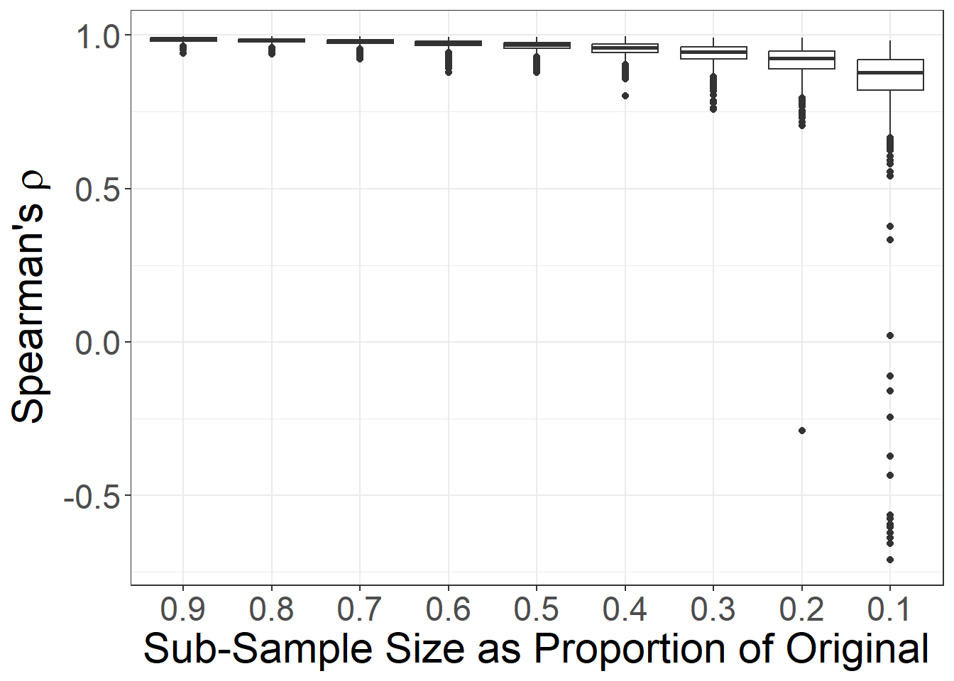
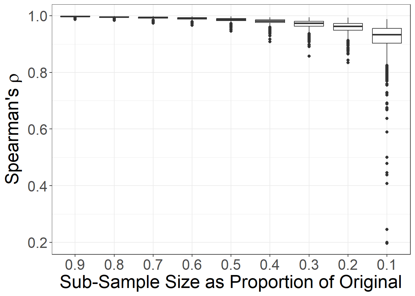
Let’s give this new function a try and calculate eigenvector centrality on the same chaco_net network object. Note that the function above has the melt function built in so the data returned are in a format required to create the plot.
# Run the function
set.seed(5609)
ev_test <- sim_missing_nodes(net = chaco_net, met = "eigenvector")

ggplot(data = ev_test) +
  geom_boxplot(aes(x = variable, y = value)) +
  xlab("Sub-Sample Size as Proportion of Original") +
  ylab(expression("Spearman's" ~ rho)) +
  theme_bw() +
  theme(
    axis.text.x = element_text(size = rel(2)),
    axis.text.y = element_text(size = rel(2)),
    axis.title.x = element_text(size = rel(2)),
    axis.title.y = element_text(size = rel(2)),
    legend.text = element_text(size = rel(1))
  )
5.4 Edges Missing at Random
In some cases, we are interested in the potential impact of missing edges rather than missing nodes. For example, if we have created a network of co-presence (based on shared ceramic types, site mentions on monuments, or some other similar data) how robust is our network to the omission of certain edges? How are different centrality metrics influenced by edge omission?
In this section, will conduct an analysis similar to that described above for assessing missing nodes. Specifically, we will sub-sample our networks by removing a fraction of edges and then test the stability of centrality measures and node position across a range of sampling fractions.
The function we defined in the previous only needs to be modified slightly to help assess edges as well. We have created a new function and associated script file that accomplishes this goal. To give you a peak beneath the hood, here are the primary lines that we needed to change. We replaced the first chunk of code here which creates a sub sample based on vcount or vertex count with a new line that uses ecount or edge count. We then further switched the induced_subgraph and instead used the delete_edges function.
Note that you should not try to evaluate the chunk of code below as it contains only portions of the larger functions described here and will return an error.
# Code from sim_missing_nodes
sub_samp <- sample(seq(1, vcount(net), prob = missing_probs),
size = round(vcount(net) * props[j], 0))
sub_net <- igraph::induced_subgraph(net, sort(sub_samp))
# Replaced code in sim_missing_edges
sub_samp <- sample(seq(1, ecount(net), prob = missing_probs),
size = round(ecount(net) * props[j], 0))
sub_net <- igraph::delete_edges(net, which(!(seq(1, ecount(net))
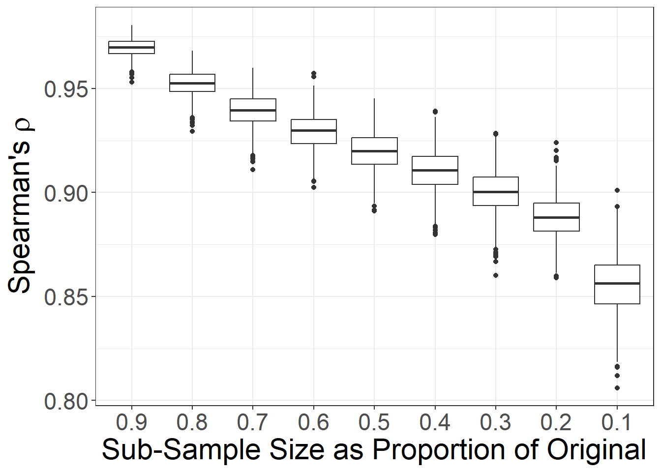
%in% sub_samp)))Let’s call our new function and assess the impact of edges missing at random on degree centrality to give this a try. We use the same default arguments for nsim and props as we did above. Since we have saved our function as a .R file, we can initialize it using the source function which lets you run all code in a specified .R file.
# First initialize the function using the .R script
source("scripts/sim_missing_edges.R")

# Run the function
set.seed(5609)
dg_edge_test <- sim_missing_edges(net = chaco_net, met = "degree")

# Visualize the results
ggplot(data = dg_edge_test) +
  geom_boxplot(aes(x = variable, y = value)) +
  xlab("Sub-Sample Size as Proportion of Original") +
  ylab(expression("Spearman's" ~ rho)) +
  theme_bw() +
  theme(
    axis.text.x = element_text(size = rel(2)),
    axis.text.y = element_text(size = rel(2)),
    axis.title.x = element_text(size = rel(2)),
    axis.title.y = element_text(size = rel(2)),
    legend.text = element_text(size = rel(1))
  )
5.5 Assessing Indivdiual Nodes/Edges
This sub-section follows along with Chapter 5.3.2 in Brughmans and Peeples (2023). In some cases we may be interested not simply in the robustness of a particular network metric to a specific kind of perturbation across all nodes or edges, but instead in the potential variability of the position or characteristics of a single node (or group of nodes) due to such perturbations. In order to explore individual nodes, we can employ similar procedures to those outlined above with a few additional modifications to our function. In this example we will use the Cibola technological similarity network. As we describe in the book, we want to assess the stability of the position of the Garcia Ranch site. Specifically, we want to know the whether or not the high betweenness centrality value of Garcia Ranch is robust to nodes missing at random in this network.
We define a new function to conduct these analyses below. This function is similar to those used above but instead of providing Spearman’s \(/rho\) values it outputs the specific rank order of the node in question across each simulation.
The function requires six pieces of information from the user:
-
net- Anigraphnetwork object. Again this is currently set up for simple networks but could easily be modified. -
target- The name of thetargetnode you wish to assess (exactly as it is written in the network object). -
prop- The proportion of nodes you wish to retain in the test. This should be a single number > 0 and < 1. -
nsim- The number of simulations. The default is 1000. -
met- This argument is used to define the metric of interest and must be one of:"betweenness","degree", or"eigenvector". If you do not specify this argument you will receive an error. -
missing_probs- This argument expects a vector that has as many values as there are nodes in the network. Each value should be a probability value between 0 and 1 (inclusive) that a node will be retained in a sub-sample of the network. You must include a probability value for thetargetnode though that node will always be retained no matter what value you use. The default for this argument isNA. If the argument isn’t specified the function assumes you are testing nodes missing at random.
Briefly how this function works is it first determines which node number corresponds with the target you wish to assess and creates nsim subgraphs that retain that target. The metric of interest is then calculated in each network and the rank order position of the target node in every network is returned. This function can be calculated either as a “missing at random” process by leaving missing_probs set to the default NA.
Let’s take a look at an example. Use these data to follow along. You can download the sim_target_node.R script here
First we read in the data:
# Read in edge list file as data frame and create network object
cibola_edgelist <-
  read.csv(file = "data/Cibola_edgelist.csv", header = TRUE)
cibola_net <-
  igraph::graph_from_edgelist(as.matrix(cibola_edgelist),
                              directed = FALSE)
Now lets initialize our function from our script using the source() function, run the function, and create a bar plot to visualize the results. Following the example in the book, we are assessing the robustness of the rank order position of Garcia Ranch in terms of betweenness centrality to nodes missing at random. Note that Garcia Ranch has the second highest centrality score in the original network:
source("scripts/sim_target_node.R")

# Run the function
set.seed(52793)
gr <- sim_target_node(
  net = cibola_net,
  target = "Garcia Ranch",
  prop = 0.8,
  nsim = 1000,
  met = "betweenness"
)

# Visualize the results
df <- as.data.frame(gr)
colnames(df) <- "RankOrder"

ggplot(df, aes(x = RankOrder)) +
  geom_bar() +
  theme_bw() +
  labs(title = " ", x = "Rank Order", y = "Count") +
  theme(
    axis.text.x = element_text(size = rel(2)),
    axis.text.y = element_text(size = rel(2)),
    axis.title.x = element_text(size = rel(2)),
    axis.title.y = element_text(size = rel(2))
  )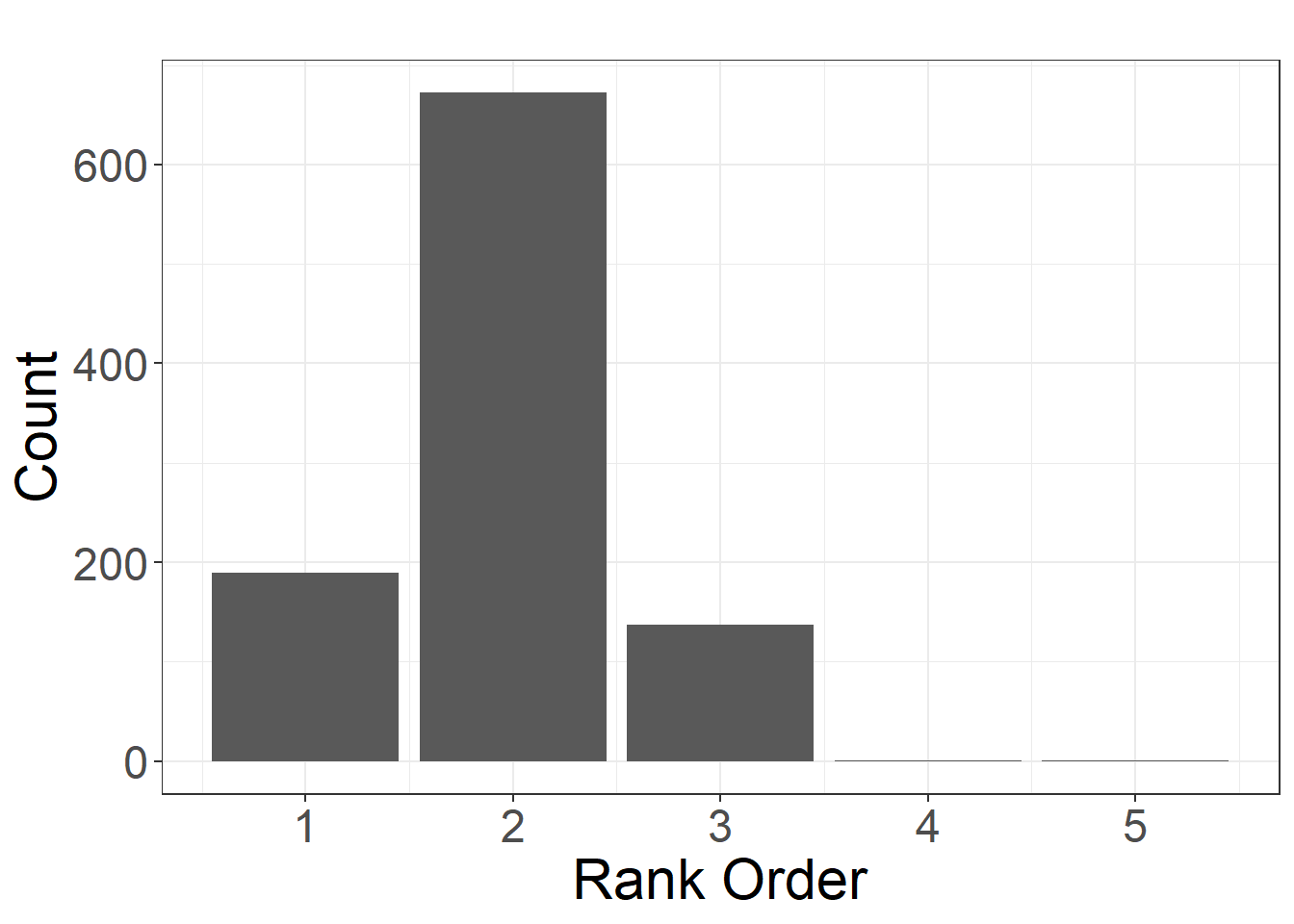
As we describe in the book, the position of Garcia Ranch as a highly central node appears to be stable to nodes missing at random. Indeed, by far the most common position for this node was 2 which is its position in the original network.
5.6 Nodes/Edges Missing Due to Biased Sampling
This sub-section follows along with Brughmans and Peeples (2023) Chapter 5.3.3. There are many contexts where we are interested in modeling data that are not missing at random but instead are influenced by some biased sampling process. For example, say we have a study area where there have been lots of general reconnaissance surveys that have recorded most of the large sites but few full coverage surveys that have captured smaller sites. In that case, we may wish to model missingness such that small sites would more likely be missing than large sites.
The sim_missing_nodes and sime_missing_edges functions we created above can both help us test the impacts of biased sampling processes. In order to do this we simply use the additional argument missing_probs. This argument requires a vector the same length as the number of nodes or edges, depending on which function you are using. This vector should contain numeric values between 0 and 1 that denote the probabilities that a node or edge will be retained in the sub-sampling effort (and must be in the same order that nodes or edges are recorded in the network object).
Let’s look under the hood to see how this change is implemented in the code. We only need to modify one line of code to include biased sampling processes. In the chunk of code below we have two lines that use the sample function. This function takes a vector of numbers and selects a sample (without replacement by default) of the specified size. If you add the argument prob it will use the vector or probabilities provided to weight the sample. That’s all there is to it.
The code chunk below is just for the purposes of demonstration and only represents part of the function so don’t try to evaluate this chunk or you’ll get an error.
# Random sampling process
sub_samp <- sample(seq(1, vcount(net)),
                   size = round(vcount(net) * props[j], 0))

# Biased sampling process
sub_samp <- sample(seq(1, vcount(net)), prob = missing_probs,
                   size = round(vcount(net) * props[j], 0))
Now, let’s try a real example using the chaco_net data again by creating a random variable to stand in for missing_probs here. We will test the impact on missing nodes. We simply create a vector of 223 random uniform numbers using the runif function to simulate probabilities associated with the 223 nodes. In practice, these probabilities could be based on site size, visibility, or any other feature you choose.
# Create 233 random numbers between 0 and 1 to stand in for
# node probabilities
set.seed(4463)
mis <- runif(223, 0, 1)
mis[1:10]
## [1] 0.6903157 0.9895447 0.3810867 0.2849476 0.2689112 0.9784197 0.8042309
## [8] 0.5805580 0.8660900 0.6179489
# Run the function
dg_test <- sim_missing_nodes(chaco_net, met = "degree", missing_probs = mis)

# Visualize the results
ggplot(data = dg_test) +
  geom_boxplot(aes(x = variable, y = value)) +
  xlab("Sub-Sample Size as Proportion of Original") +
  ylab(expression("Spearman's" ~ rho)) +
  theme_bw() +
  theme(
    axis.text.x = element_text(size = rel(2)),
    axis.text.y = element_text(size = rel(2)),
    axis.title.x = element_text(size = rel(2)),
    axis.title.y = element_text(size = rel(2)),
    legend.text = element_text(size = rel(1))
  )
5.6.1 Resampling with Incidence Matrices
In the book, we illustrate our approach to biased sampling using the co-authorship network data. In this case we start with an incidence matrix of publications and authors and we want to assess the potential impact of missing publications on the network of authors. Since we gathered these data from digital repositories and citations, it is likely that we are missing some publications and it is reasonable to assume that we would be more likely to miss older publications than newer ones given the inclusion of newer publications in searchable digital indexes. Thus, in this example we want to assess missingness such that newer publications are more likely to be retained than older ones in our sample. We compare this to missing at random to assess how these results relate to one another.
First we need to provide two data files. The first is the bibliographic attribute data which includes date, publication type, and other information on each publication designated by a unique identifier. The second is an incidence matrix of publications denoted by unique identifier (rows) and authors (columns). We read this into R and then create an adjacency matrix of author to author connections using matrix algebra (multiply the incidence matrix by the transpose of the incidence matrix), convert it into a igraph network object and then calculate betweenness centrality for all nodes. We plot a simple network node link diagram to visualize these data.
# Read in publication and author attribute data
bib <- read.csv("data/biblio_attr.csv")
bib[1:3, ]
## Key Item.Type
## 1 FUV8A7JK journalArticle
## 2 C7MRVHWA bookSection
## 3 3EG6T4P6 journalArticle
## Publication.Title
## 1 Archaeological Review from Cambridge
## 2 Network analysis in archaeology. New approaches to regional interaction
## 3 American Antiquity
## Publication.Year Authors
## 1 2014 Stoner, Jo
## 2 2013 Isaksen, Leif
## 3 1991 Peregrine, Peter
# Read in incidence matrix of publication and author data
bib_dat <-
  as.matrix(read.table(
    "data/biblio_dat2.csv",
    header = TRUE,
    row.names = 1,
    sep = ","
  ))

# Create adjacency matrix from incidence matrix using matrix algebra
bib_adj <- t(bib_dat) %*% bib_dat
# Convert to igraph network object removing self loops (diag=FALSE)
bib_net <- igraph::graph_from_adjacency_matrix(bib_adj,
                                               mode = "undirected",
                                               diag = FALSE)
# Calculate Betweenness Centrality
bw_all <- igraph::betweenness(bib_net)

# Plot network with nodes scaled based on betweenness
set.seed(346)
ggraph(bib_net, layout = "fr") +
  geom_edge_link0(width = 0.2) +
  geom_node_point(shape = 21,
                  aes(size = bw_all * 5),
                  fill = "gray",
                  alpha = 0.75) +
  theme_graph() +
  theme(legend.position = "none")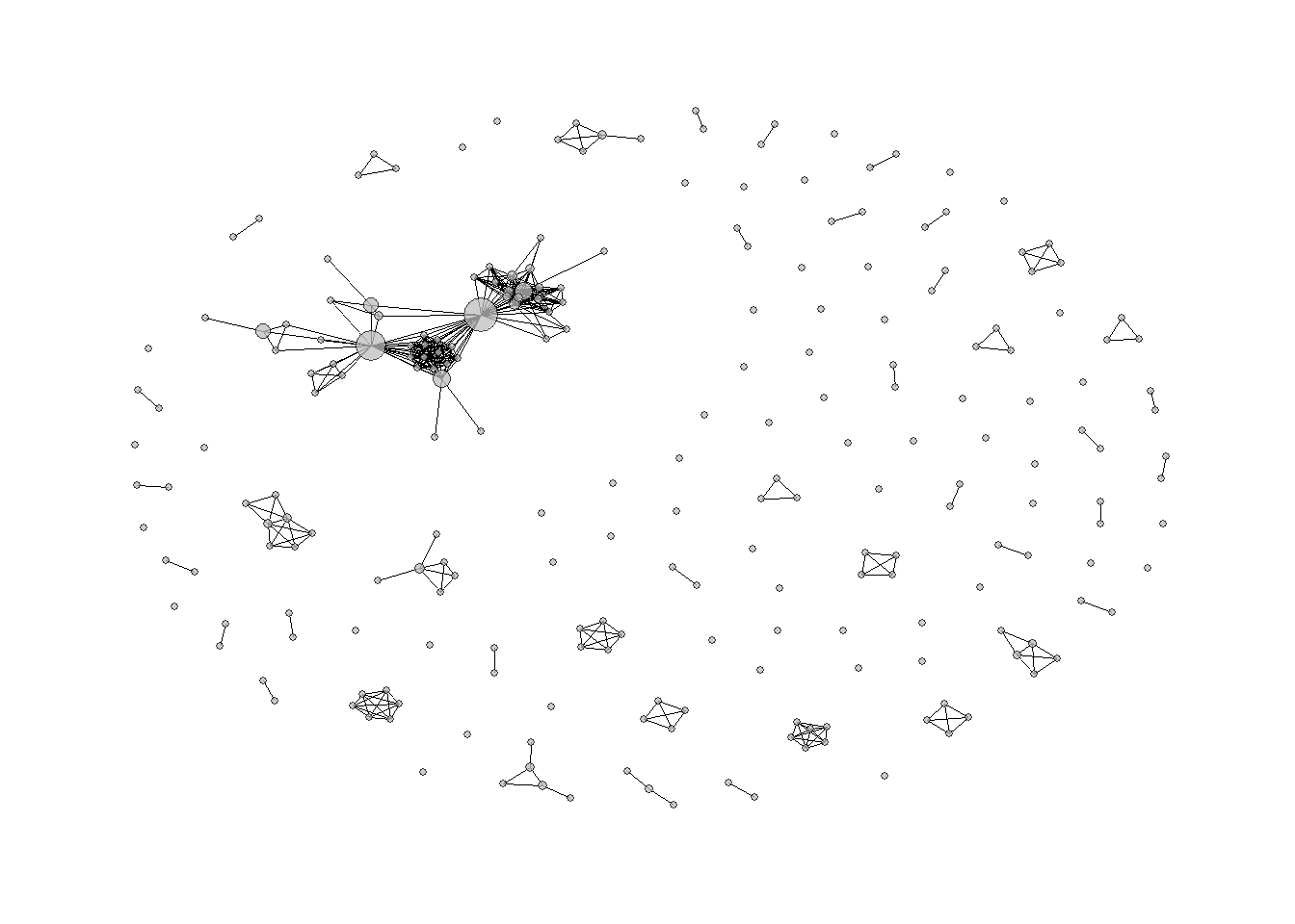
Although it may at first seem like we could use the same function we used previously to assess missing nodes, there are some key differences in the organization of data in this network that won’t permit that. Specifically, we are interested in nodes (authors) missing at random, but we we want to model probabilities associated with publications. This is a slightly more complicated procedure because the function needs both the network object and the incidence matrix from which it was generated so that the sub-networks can be defined inside the function. We have created a sim_missing_inc function (simulating missing data using an incidence matrix) that conducts this task.
This function requires five specific pieces of information from the user:
-
net- You must include a network object inigraphformat. We use a simple network here but the code could be modified for directed or valued networks. -
inc- You must also include an incidence matrix (as an R matrix object) which describes the relationships between. The incidence matrix needs to have unique row names and column names. The mode you are interested in assessing should be the columns (in other words if you are interested in authors missing at random authors should be represented by columns and publications by rows). -
nsim- You must specify the number of simulations to perform. The default is 1000. -
props- You must specify the proportion of nodes to be retained for each set ofnsimruns. This should be provided as a vector of proportions ranging from > 0 to 1. By default, the script will calculate a 0.9 sub-sample all the way down to a 0.1 sub-sample at 0.1 intervals usingprops=c(0.9,0.8,0.7,0.6,0.5,0.4,0.3,0.2,0.1). -
lookup_dat- Finally, you need to provide a data frame or matrix that contains two columns. The first column should be the unique name for each row in the incidence matrix (publication key in this case). The second column should include a numeric value between 0 and 1 which indicates the probability that each row will be retained in the resampling process. If you include nothing formissing_probsthe function will remove columns at random with an equal probability for each.
In our example here, we must first calculate the data we need to provide for the missing_probs argument above. To do this we simply take the vector of publication years in the bib object we read in and rescale them such that the maximum value (most recent publication) equals 1 and older publications are less than 1. This will mean that older publications will more often be removed in our random sub-samples than newer ones as outlined in the example in the book.
Note that the script provided here is focused on assessing whichever
category of nodes is represented by columns in the original incidence
matrix. You would need to modify this code to use it for an incidence
matrix where rows or your target or simply use the t()
transpose function to place columns in the target position.
# Create a data frame of all unique combinations of publication code
# and year from attributes data
lookup <- unique(bib[, c(1, 4)])
# Assign a probability for a publication to be retained inverse to
# the year it was published
lookup_prob <-
  (lookup$Publication.Year - min(lookup$Publication.Year)) /
  (max(lookup$Publication.Year) - min(lookup$Publication.Year))

# Create data frame with required output. We have added a sort function
# here to ensure that the order of probabilities in lookup_dat is the
# same as the order of rows in the incidence matrix. You will get
# spurious results if you do not ensure these are the same.
lookup_dat <- sort(data.frame(Key = lookup[,1], prob = lookup_prob))
head(lookup_dat)
## Key prob
## 117 24QNVV37 0.9583333
## 86 29GVMCNZ 0.0625000
## 81 2QC8N5RN 1.0000000
## 112 2QU9ZNUG 0.8125000
## 126 2T8HPW5E 0.9583333
## 18 37TC37D2 1.0000000With the probabilities of retention for missing_probs in place, we can then call source code for our sim_missing_inc.R script and run the function. Following the example in the book we run the function for nsim = 1000 and for 3 sampling fractions (0.9, 0.8, 0.7) with the metric of interest as betweenness. Let’s first run the function for our “probability by date” biased sampling process.
source("scripts/sim_missing_inc.R")

# Run function
set.seed(4634)
bib_bias <- sim_missing_inc(
  net = bib_net,
  inc = bib_dat,
  missing_probs = lookup_dat$prob,
  props = c(0.9, 0.8, 0.7),
  met = "betweenness",
)
head(bib_bias)
## variable value
## 1 0.9 0.9747220
## 2 0.9 0.9608842
## 3 0.9 0.9999614
## 4 0.9 0.9999803
## 5 0.9 0.9760737
## 6 0.9 0.9999803Next we want to run the function again to simulate nodes missing at random. All we need to do is change the missing_probs argument to NA (or exclude that argument altogether). Let’s run it:
# Run the function
set.seed(4363)
bib_rand <- sim_missing_inc(
  net = bib_net,
  inc = bib_dat,
  missing_probs = NA,
  props = c(0.9, 0.8, 0.7),
  met = "betweenness"
)
head(bib_rand)
## variable value
## 1 0.9 0.9817859
## 2 0.9 0.9804552
## 3 0.9 0.9818085
## 4 0.9 0.8911948
## 5 0.9 0.8733779
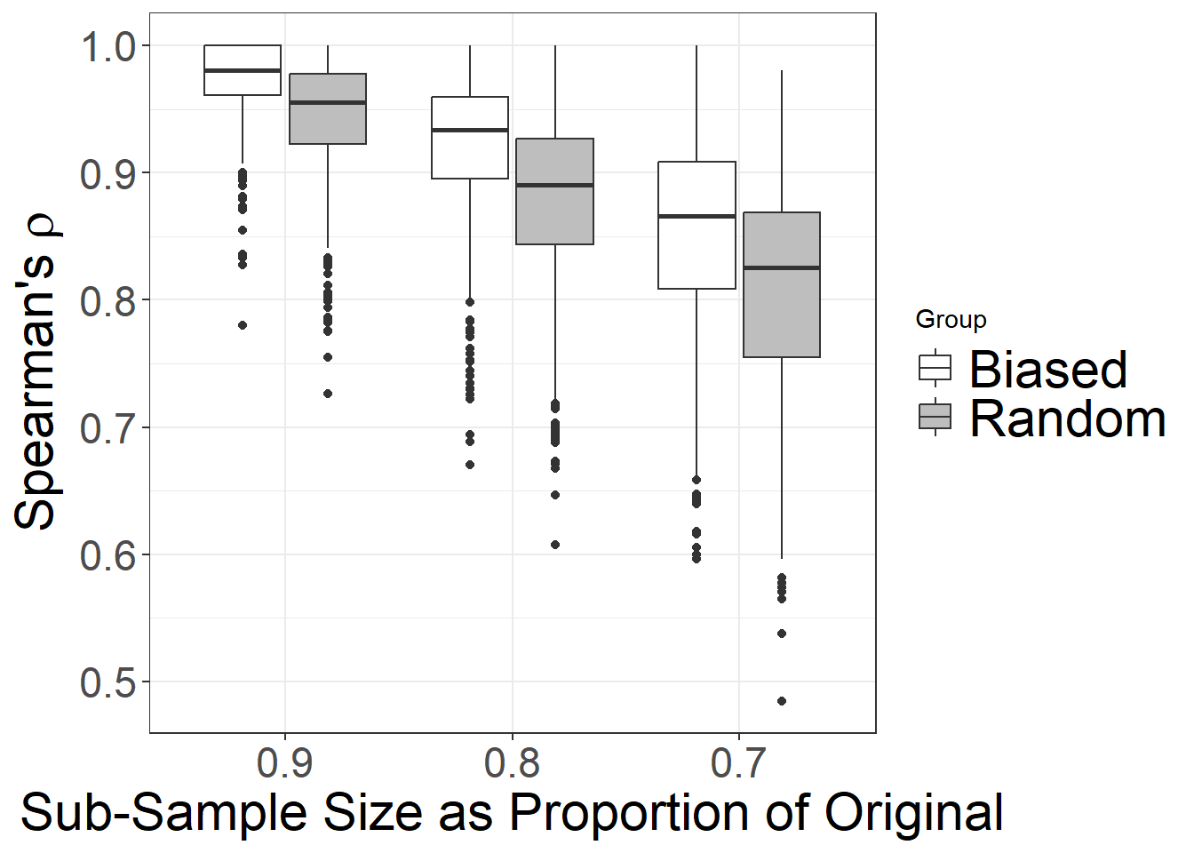
## 6 0.9 1.0000000Now we can combine the results into a single data frame and plot them as paired box plots for comparison. In order to create paired box plots it is easiest to create a single data frame that contains the results of both runs above. We combine these and add a new column called “Treatment” that specifies for each row in the data frame whether it was part of the Random or Biased sample.
# Add a variable denoting which sample design it came from
bib_rand$treatment <- rep("Random", nrow(bib_rand))
bib_bias$treatment <- rep("Biased", nrow(bib_bias))

# Bind into a single data frame, convert sampling faction to factor
# and change order of levels for plotting
df <- rbind(bib_rand, bib_bias)
df$variable <- as.factor(df$variable)
df$variiable <- factor(df$variable, levels = c("0.9", "0.8", "0.7"))

# Plot the results
ggplot(data = df) +
  geom_boxplot(aes(x = variable, y = value, fill = treatment)) +
  scale_fill_manual(values = c("white", "gray"), name = "Group") +
  xlab("Sub-Sample Size as Proportion of Original") +
  ylab(expression("Spearman's" ~ rho)) +
  theme_bw() +
  theme(
    axis.text.x = element_text(size = rel(2)),
    axis.text.y = element_text(size = rel(2)),
    axis.title.x = element_text(size = rel(2)),
    axis.title.y = element_text(size = rel(2)),
    legend.text = element_text(size = rel(2))
  )
5.7 Edge Probability Modeling
In this section we take inspiration from some recent work in the area of “Dark Networks” (see Everton 2012) or the investigation of illicit networks. In this field, a number of methods have recently been developed that allow researchers to more directly incorporate assessments of the reliability of specific edges into analyses. This can be done in a number of different ways. Perhaps the most common approach for networks based on data gathered from intelligence sources (such as studies of terrorist networks) is to qualitatively assign different levels of confidence to ties between pairs of actors using an ordinal scale determined based on the source of the information (reliable, usually reliable,… unreliable). This ordinal scale of confidence can then be converted into a probability (from 0 to 1) and that probability value could be used to inform the creation of a range of “possible” networks given the underlying data.
We are not aware of any archaeological examples where edges have been formally qualitatively assigned “confidence levels” in exactly this way, but we think there are potential applications of this method. For example, we could define a network where we assign a low probability of a tie between two archaeological sites if they share an import from a third site/region and a higher probability for a tie between two sites if they share imports from each others’ region. Importantly, such methods can be used to combine information from different sources into a single assessment of the probability of connection.
Since we do not have any data structured in exactly this way, we will use a small simulated data set that consists of and edge list with weights. Use this file to follow along. This is a simple edge list with probability values assigned to each edge at values of 0.2, 0.4, 0.6, 0.8, and 1.0.
Let’s read in the data and plot it:
# Read in edge_list
sim_edge <- as.matrix(read.csv("data/sim_edge.csv",
                     header = T, row.names = 1))

# Create network object and assign edge weights and node names
sim_net <- igraph::graph_from_edgelist(sim_edge[, 1:2])
E(sim_net)$weight <- sim_edge[order(sim_edge[, 3]), 3]
V(sim_net)$name <- seq(1:20)

# Create color ramp palette
edge_cols <- colorRampPalette(c("gray", "darkblue"))(5)

# Plot the resulting network
set.seed(4364672)
ggraph(sim_net, layout = "fr") +
  geom_edge_link0(aes(width = E(sim_net)$weight * 5),
                  edge_colour = edge_cols[E(sim_net)$weight * 5],
                  show.legend = FALSE) +
  geom_node_point(shape = 21,
                  size = igraph::degree(sim_net) + 3,
                  fill = "red") +
  geom_node_text(
    aes(label = as.character(name)),
    col = "white",
    size = 3.5,
    repel = FALSE
  ) +
  theme_graph()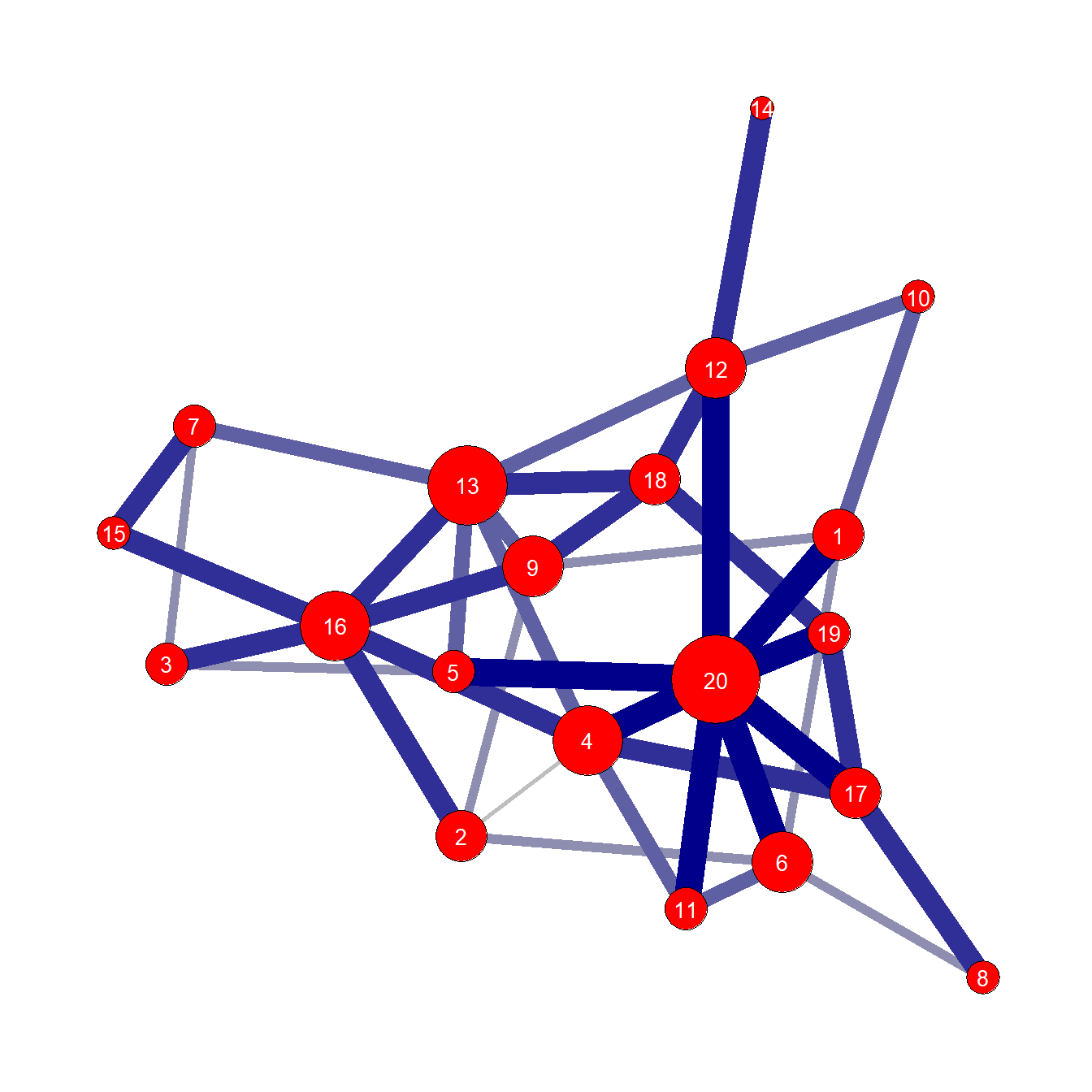
In the next chunk of code we define a function that iterates over every edge in the simulated network we just created and defines each edge as either present or absent using a simple random binomial with the probability set by the edge weight as described above. The output of this function (edge_prob) is a list object that contains nsim igraph network objects that are candidate networks of the original.
In order to extract values of interest from these candidate networks, we created another function called compile_stat. This function iterates over all nsim networks in the net_list list object and calculates the centrality metric of interest in this case returning the results as a simple matrix. It is then possible to compare things like average degree or the distribution of degree for particular nodes across all of the candidate networks. We have placed these two functions in an additional script file called edge_prob.R which you can download to use and modify on your own.
# Define function for assessing and retaining edges based on edge
# weight probabilities
edge_prob <- function(net, nsim = 1000, probs) {
  net_list <- list()
  for (i in 1:nsim) {
    sub_set <- NULL
    for (j in 1:ecount(net)) {
      temp <- rbinom(1, 1, prob = probs[j])
      if (temp == 1) {
        sub_set <- c(sub_set, j)
      }
    }
    net_list[[i]] <-
      igraph::delete_edges(net, which(!(seq(1, ecount(
        net
      ))
      %in% sub_set)))
  }
  return(net_list)
}

# Define function for assessing statistic of interest
compile_stat <- function(net_list, met) {
  out <- matrix(NA, vcount(net_list[[1]]), length(net_list))
  for (i in seq_len(length(net_list))) {
    # Select measure of interest based on met and calculate(same as above)
    if (met == "degree") {
      out[, i] <- igraph::degree(net_list[[i]])
    }
    else  {
      if (met == "betweenness") {
        out[, i] <- igraph::betweenness(net_list[[i]])
      }
      else {
        if (met == "eigenvector") {
          out[, i] <- igraph::eigen_centrality(net_list[[i]])$vector
        }
      }
    }
  }
  return(out)
}
Now we run the edge_prob function for nsim = 1000 and display a few candidate networks.
el_test <- edge_prob(sim_net, nsim = 1000, probs = sim_edge[, 3])

set.seed(9651)
comp1 <- ggraph(el_test[[1]], layout = "fr") +
  geom_edge_link0(aes(width = E(el_test[[1]])$weight),
                  edge_colour = edge_cols[E(el_test[[1]])$weight * 5],
                  show.legend = FALSE) +
  geom_node_point(shape = 21,
                  size = igraph::degree(el_test[[1]]),
                  fill = "red") +
  geom_node_text(
    aes(label = as.character(name)),
    col = "white",
    size = 2.5,
    repel = FALSE
  ) +
  theme_graph()

comp2 <- ggraph(el_test[[2]], layout = "fr") +
  geom_edge_link0(aes(width = E(el_test[[2]])$weight),
                  edge_colour = edge_cols[E(el_test[[2]])$weight * 5],
                  show.legend = FALSE) +
  geom_node_point(shape = 21,
                  size = igraph::degree(el_test[[2]]),
                  fill = "red") +
  geom_node_text(
    aes(label = as.character(name)),
    col = "white",
    size = 2.5,
    repel = FALSE
  ) +
  theme_graph()

comp3 <- ggraph(el_test[[3]], layout = "fr") +
  geom_edge_link0(aes(width = E(el_test[[3]])$weight),
                  edge_colour = edge_cols[E(el_test[[3]])$weight * 5],
                  show.legend = FALSE) +
  geom_node_point(shape = 21,
                  size = igraph::degree(el_test[[3]]),
                  fill = "red") +
  geom_node_text(
    aes(label = as.character(name)),
    col = "white",
    size = 2.5,
    repel = FALSE
  ) +
  theme_graph()

ggarrange(comp1, comp2, comp3)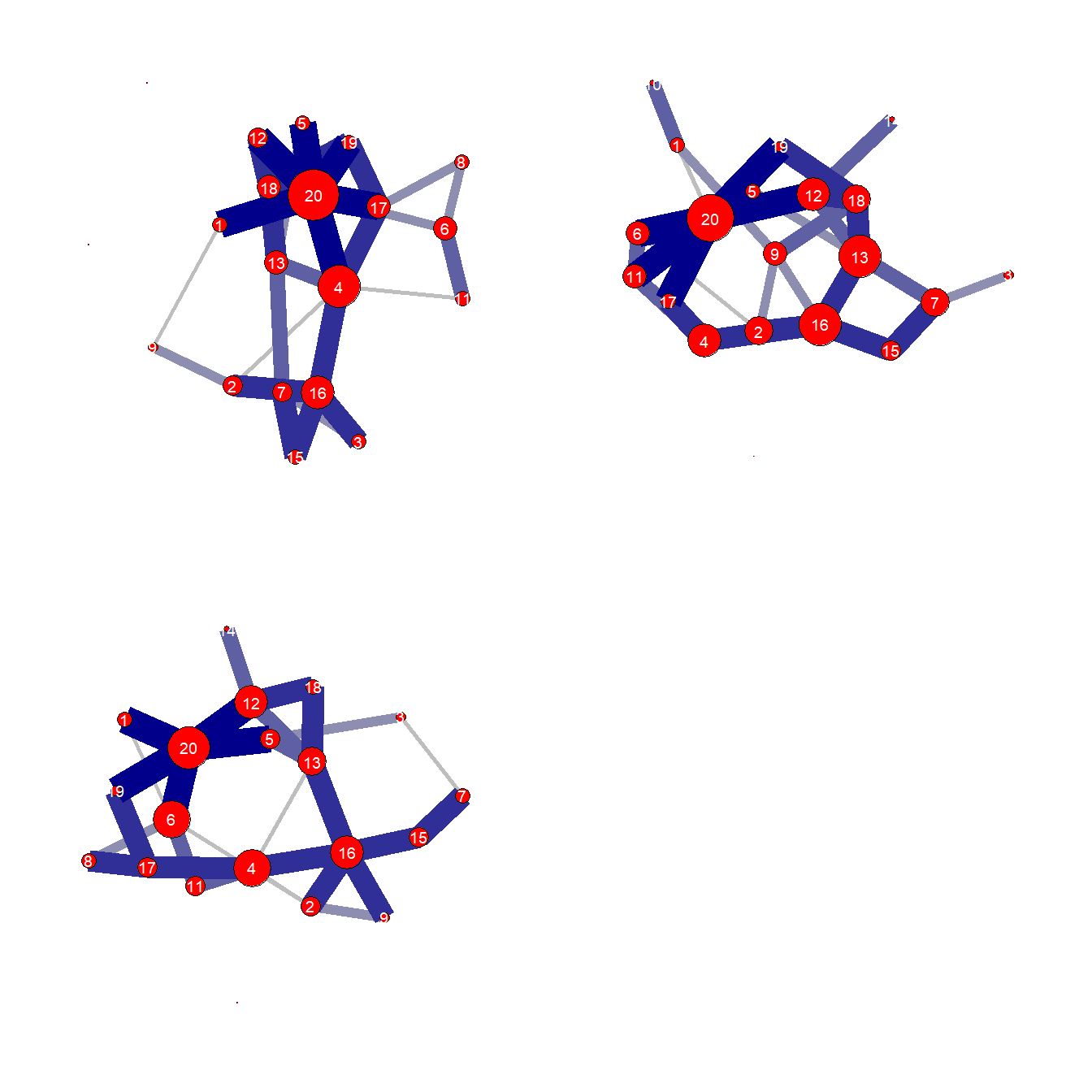
We then use the compile_stat function to assess degree centrality for one particular node, displaying a histogram of values with mean indicated.
dg_stat <- compile_stat(el_test, met = "degree")

dg_20 <- data.frame(val = dg_stat[20, ])

ggplot(dg_20, aes(val)) +
  geom_histogram(binwidth = 1) +
  xlab("Degree Centrality of Node 20") +
  geom_vline(xintercept = mean(dg_20$val), col = "red") +
  theme_bw()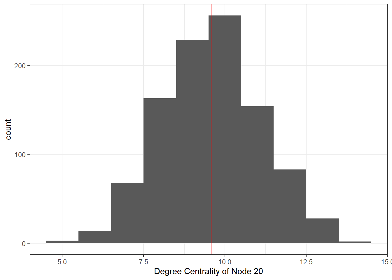
5.7.1 Edge Probability and Similarity Networks
One area of archaeological network research where the edge probability modeling approach outlined above may be of use relates to similarity networks. Many similarity networks used in archaeology are built such that the edge weights are scaled between 0 and 1. These edge weights could be thought of as “probabilities” just as we saw with the simulated example above. Indeed, this conforms with the frequent interpretation of similarity values as relating to probabilities of interaction in numerous network studies (e.g., Mills et al. 2013a, 2013b, 2015; Golitko and Feinman 2015; Golitko et al. 2012, etc.).
Let’s take a look at an example using a weighted similarity network generated using the Cibola technological similarity data used above. Download the RData file here to follow along.
load("data/Cibola_wt.RData")

# View first few edge weights in network object
E(cibola_wt)$weight[1:10]
## [1] 0.7050691 0.7757143 0.8348214 0.8656783 0.8028571 0.7329193 0.7509158
## [8] 0.8441558 0.7857143 0.8102919Now let’s plot a couple of the candidate networks:
# Precompute layout
set.seed(9631)
xy <- layout_with_fr(cibola_wt)

# Example 1
comp1 <- ggraph(sim_nets[[1]],
                layout = "manual",
                x = xy[, 1],
                y = xy[, 2]) +
  geom_edge_link() +
  geom_node_point(shape = 21,
                  size = igraph::degree(sim_nets[[1]]) / 3,
                  fill = "red") +
  theme_graph()

# Example 2
comp2 <- ggraph(sim_nets[[2]],
                layout = "manual",
                x = xy[, 1],
                y = xy[, 2]) +
  geom_edge_link() +
  geom_node_point(shape = 21,
                  size = igraph::degree(sim_nets[[2]]) / 3,
                  fill = "red") +
  theme_graph()

# Example 3
comp3 <- ggraph(sim_nets[[3]],
                layout = "manual",
                x = xy[, 1],
                y = xy[, 2]) +
  geom_edge_link() +
  geom_node_point(shape = 21,
                  size = igraph::degree(sim_nets[[3]]) / 3,
                  fill = "red") +
  theme_graph()

ggarrange(comp1, comp2, comp3)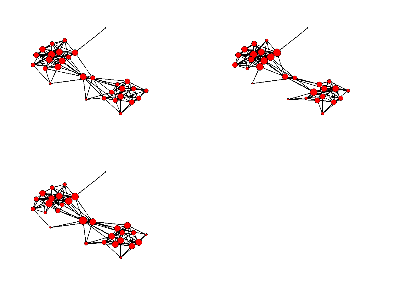
bw_test <- compile_stat(sim_nets, met = "betweenness")

bw_10 <- data.frame(val = bw_test[10, ])

ggplot(bw_10, aes(val)) +
  geom_histogram() +
  xlab("Betweenness Centrality of Node 10") +
  geom_vline(xintercept = mean(bw_10$val), col = "red") +
  theme_bw()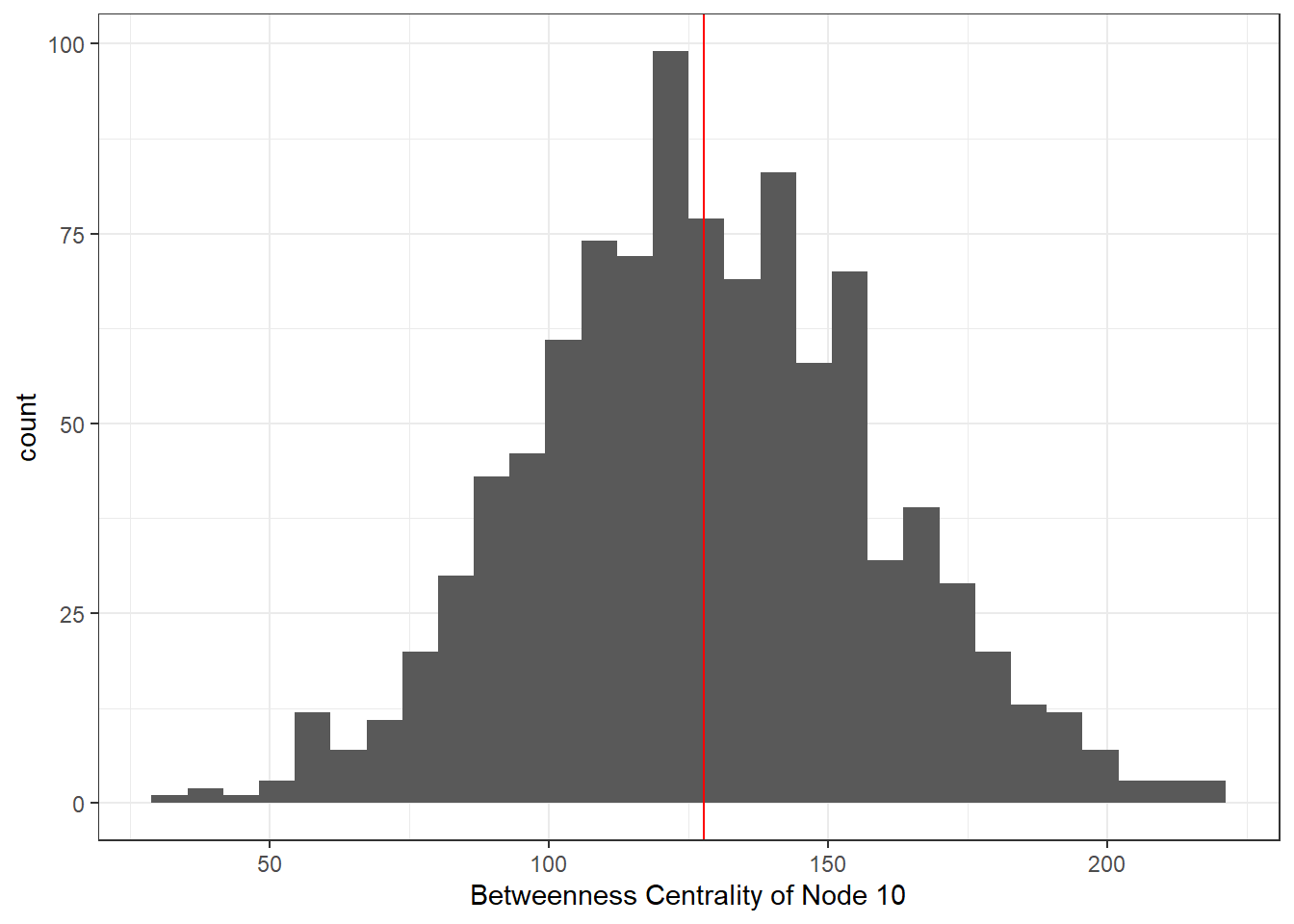
5.8 Uncertainty Due to Small or Variable Sample Size
This section follows Brughmans and Peeples (2023) Chapter 5.3.5 to provide an example of how you can use the simulation approach outlined here to assess sampling variability in the frequency data underlying archaeological networks. In this example, we use apportioned ceramic frequency data from the Chaco World portion of the Southwest Social Networks database. You can download the data here to follow along.
The goal of this sub-section is to illustrate how you can use a bootstrapping approach to assess variability in network properties based on sampling error in the raw data underlying archaeological networks. In our example based on ceramic similarity networks here this involves creating a large number of random replicates of each row of our raw ceramic data with sample size held constant (as the observed sample size for that site) and with the probabilities that a given sherd will be a given type determined by the underlying multinomial frequency distribution of types at that site. In other words, we pull a bunch of random samples from the site with the probability that a given sample is a given type determined by the relative frequency of that type in the actual data. Once this procedure has been completed, we can then assess centrality metrics or any other graph, node, or edge level property and determine the degree to which absolute values and relative ranks are potentially influenced by sampling error.
There are many ways to set up such a resampling procedure and many complications (for example, how do we deal with limited diversity of small samples?). For the purposes of illustration here, we will implement a very simple procedure where we simply generate new samples of a fixed size based on our observed data and determine the degree to which our network measures are robust to this perturbation. In the chunk of code below we create 1000 replicates based on our original ceramic data.
The following chunk of code first reads in the ceramic data, converts it to a Brainerd-Robinson similarity matrix and then defines a function called sim_samp_error which creates nsim random replicates of the ceramic data, converts them to similarity matrices, and outputs those results as a list object. You can download the script for the fucnction below here.
# Read in raw ceramic data
ceramic <-
read.csv(file = "data/AD1050cer.csv",
header = TRUE,
row.names = 1)
# Convert to proportion
ceramic_p <- prop.table(as.matrix(ceramic), margin = 1)
# Convert to Brainerd-Robinson similarity matrix
ceramic_br <- ((2 - as.matrix(vegan::vegdist(ceramic_p,
method = "manhattan"))) / 2)
# Create function for assessing impact of sampling error on
# weighted degree for similarity network
sim_samp_error <- function(cer, nsim = 1000) {
sim_list <- list()
for (i in 1:nsim) {
data_sim <- NULL
# the for-loop below creates a random multinomial replicate
# of the ceramic data
for (j in seq_len(nrow(cer))) {
data_sim <-
rbind(data_sim, t(rmultinom(1, rowSums(cer)[j], prob = cer[j, ])))
}
# Convert simulated data to proportion, create similarity matrix,
# calculate degree, and assess correlation
temp_p <- prop.table(as.matrix(data_sim), margin = 1)
sim_list[[i]] <- ((2 - as.matrix(vegan::vegdist(temp_p,
method = "manhattan"))) / 2)
}
return(sim_list)
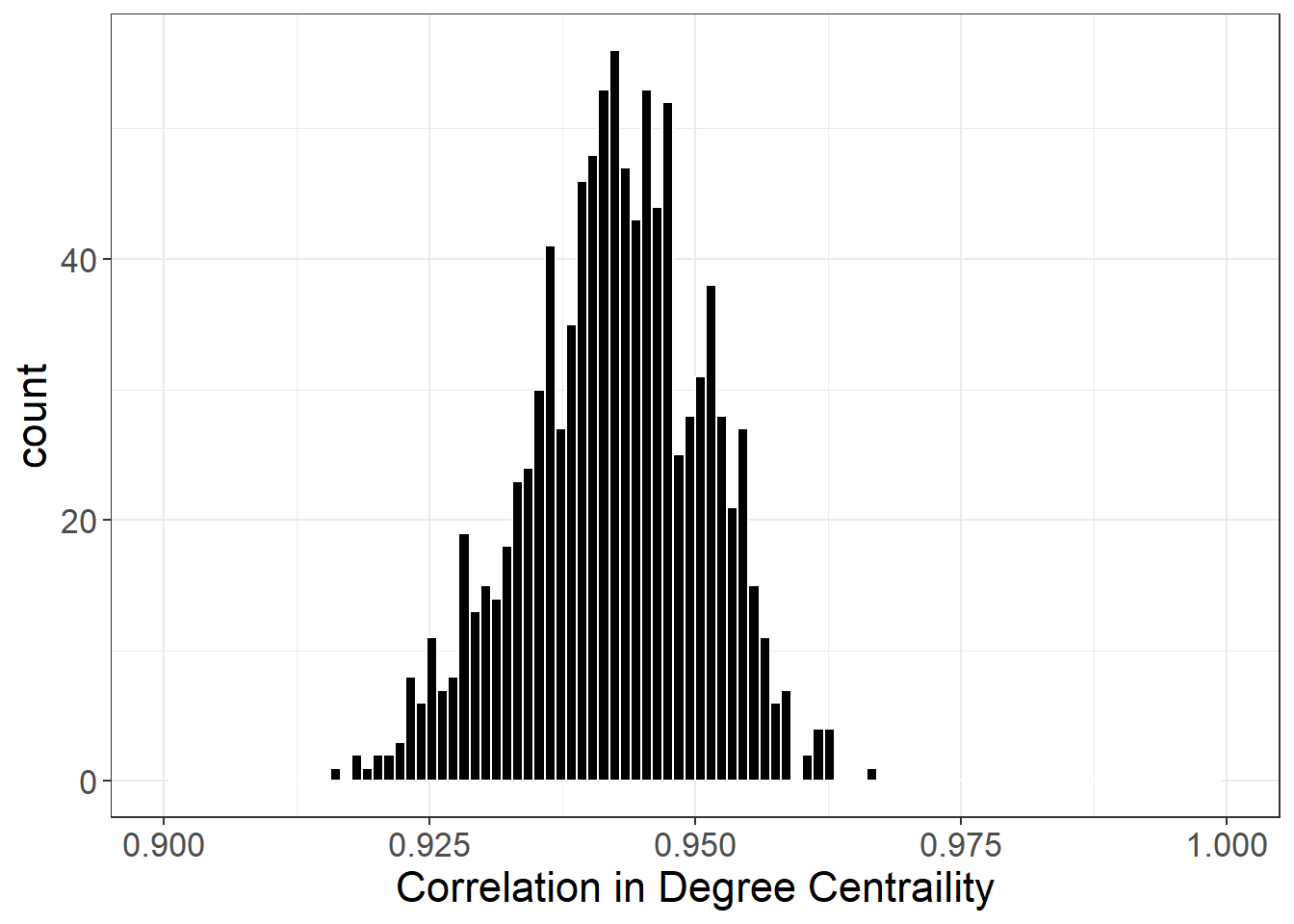
}The following chunk of code runs the sim_samp_error function defined above for our Chaco ceramic data and then defines a new function called sim_cor which takes the output of sim_samp_error and the original ceramic similarity matrix (ceramic_BR) and calculates weighted degree centrality and the Spearman’s \(\rho\) correlations between the original similarity matrix and each random replicate. This sim_cor script could be modified to use any network metric that outputs a vector. Once these results are returned we visualize the results as a histogram.
Note that this could take several seconds to a few minutes depending on your computer.
set.seed(4634)
sim_nets <- sim_samp_error(cer = ceramic, nsim = 1000)

sim_cor <- function(sim_nets, sim) {
  # change this line to use a different metric
  dg_orig <- rowSums(sim)
  dg_cor <- NULL
  for (i in seq_len(length(sim_nets))) {
    # change this line to use a different metric
    dg_temp <- rowSums(sim_nets[[i]])
    dg_cor[i] <-
      suppressWarnings(cor(dg_orig, dg_temp, method = "spearman"))
  }
  return(dg_cor)
}

dg_cor <- sim_cor(sim_nets, ceramic_br)

df <- as.data.frame(dg_cor)

ggplot(df, aes(x = dg_cor)) +
  geom_histogram(bins = 100, color = "white", fill = "black") +
  theme_bw() +
  scale_x_continuous(name = "Correlation in Degree Centraility",
                     limits = c(0.9, 1)) +
  theme(
    axis.text.x = element_text(size = rel(1.5)),
    axis.text.y = element_text(size = rel(1.5)),
    axis.title.x = element_text(size = rel(1.5)),
    axis.title.y = element_text(size = rel(1.5)),
    legend.text = element_text(size = rel(1.5))
  )
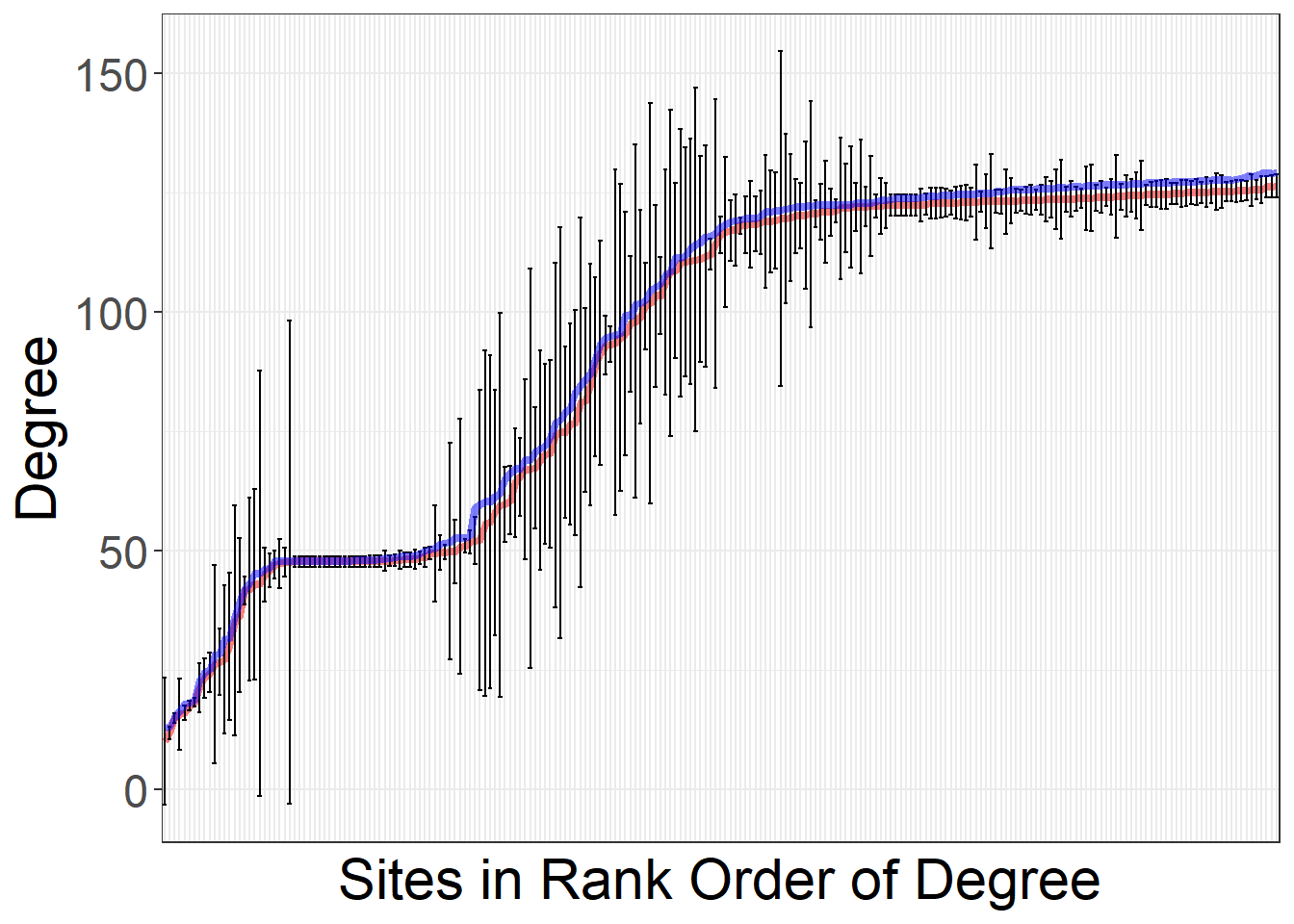
As described in Chapter 5.3.5, in some cases we want to observe patterns of variation due to sampling error for individual sites or sets of sites. In the next chunk of code we illustrate how to produce figure 5.14 from the Brughmans and Peeples (2023) book. Specifically, this plot consists of a series of line plots where the x axis represents each node in the network ordered by degree centrality in the original observed network. For each node there is a vertical line which represents the 95% confidence interval around degree across the nsim random replicates produced to evaluate sampling error. The blue line represents degree in the original network and the red line represents median degree in the resampled networks.
To create this plot, we first iterate through every object in sim_nets and calculate weighted degree centrality and then add that to a two-column matrix along with a node id. Once we have done this for all simulations, we use the summarise function to calculate the mean, median, max, min, and confidence interval (95%). We then plot the observed values of degree in blue, the mean values in red, and the confidence intervals as black vertical bars for each node. The nodes are sorted from low to high degree centrality in the original network.
# Create data frame containing degree and site id for nsim random
# similarity matrices
df <- matrix(NA, 1, 2) # define empty matrix
# calculate degree centrality for each random run and bind in
# matrix along with id
for (i in seq_len(length(sim_nets))) {
  temp <- cbind(seq(1, nrow(sim_nets[[i]])), rowSums(sim_nets[[i]]))
  df <- rbind(df, temp)
}
df <- as.data.frame(df[-1, ]) # remove first row in initial matrix
colnames(df) <- c("site", "degree") # add column names

# Use summarise function to create median, confidence intervals,
# and other statistics for degree by site.
out <- df %>%
  group_by(site) %>%
  dplyr::summarise(
    Mean = mean(degree),
    Median = median(degree),
    Max = max(degree),
    Min = min(degree),
    Conf = sd(degree) * 1.96
  )
out$site <- as.numeric(out$site)
out <- out[order(rowSums(ceramic_br)), ]

# Create data frame of degree centrality for the original ceramic
# similarity matrix
dg_wt <- as.data.frame(rowSums(ceramic_br))
colnames(dg_wt) <- "dg.wt"

# Plot the results
ggplot() +
  geom_line(
    data = out,
    aes(
      x = reorder(site, Median),
      y = Median,
      group = 1
    ),
    col = "red",
    lwd = 1.5,
    alpha = 0.5
  ) +
  geom_errorbar(data = out, aes(
    x = reorder(site, Median),
    ymin = Median - Conf,
    ymax = Median + Conf
  )) +
  geom_path(
    data = sort(dg_wt),
    aes(x = order(dg.wt), y = dg.wt),
    col = "blue",
    lwd = 1.5,
    alpha = 0.5
  ) +
  theme_bw() +
  ylab("Degree") +
  scale_x_discrete(name = "Sites in Rank Order of Degree") +
  theme(
    axis.text.x = element_blank(),
    axis.ticks.x = element_blank(),
    axis.text.y = element_text(size = rel(2)),
    axis.title.x = element_text(size = rel(2)),
    axis.title.y = element_text(size = rel(2)),
    legend.text = element_text(size = rel(2))
  )